
More efficient buildings lead to lower rooftop solar returns
Why the order of your decarbonization projects matters

Built environment decarbonization is a long and complex process that will keep us busy for much of this century. When organizations first start looking into decarbonizing their portfolios, they quickly realize there’s a limited budget and many potential projects to optimize energy consumption and reduce emissions. A natural question quickly comes up: what should we do first, and where? The answer isn’t trivial, because every building in a portfolio is unique, consumption often changes over time, and each project influences the potential impact of any other project at the same site.
In this post, I want to exemplify this by showing how the economics of a rooftop PV system can change drastically when an Energy Conservation Measure (ECM) is implemented in a building.
At Ento, I’ve been working for quite some time on a tool to predict the optimal decarbonization roadmap for a certain building or portfolio. One of the challenges with these types of tools is that the order in which projects are implemented is not interchangeable. For instance, consider a building where we could:
Convert existing lighting to more efficient LED fixtures
Replace a gas boiler used for space heating with a heat pump
Upgrade to better-insulated windows
Install a rooftop PV system
Each action has a certain impact on final energy consumption and carbon emissions, but they also influence one another:
LED installation will reduce the electricity demand
Replacing the gas boiler with a heat pump will eliminate gas consumption but increase electricity consumption.
Replacing windows with more insulated ones lowers the energy required for space heating.
A rooftop PV system produces electricity that can be self-consumed or exported to the grid depending on demand during production hours.
Self-consuming PV-produced electricity is almost always more economically profitable than injecting it into the grid, which means the optimal size for a rooftop system depends heavily on the building’s load profile. Because various measures, such as lighting retrofits or heating system changes, affect that load, we need to carefully consider their impact when designing the rooftop PV system.
To illustrate this, I will consider the same building we’ve used in past tutorials, a large facility located in Washington, DC. In this building, a large ECM was implemented, and through several tutorials, we’ve been evaluating its impact on the building load. It’s also the building we used as an example for calculating the optimal PV size based on the pre-ECM electricity consumption.
In this tutorial, we will consider the same building and simulated production data. The difference is that we will match that data with the post-ECM consumption to see how the electricity self-consumption, self-sufficiency, and the annual return on investment change.
We’ll require a few things to get our final result, but I’ll skip the code snippets that were explained in previous posts. You can find all our previously published tutorials at this link, but if you need a quick recap:
In tutorials [1], [2], and [3] we built a counterfactual model to estimate energy efficiency savings from an implemented ECM
In tutorial [4] we extrapolated those savings to one full year from only six months of data
In tutorial [5] we simulated the solar energy produced by a rooftop PV system installed on the building.
In tutorial [6] we matched the production with the building consumption to calculate self-sufficiency and self-consumption ratios.
In tutorial [7] we compared the energy production simulated with pvlib with the one provided from the Google Solar API for the same location
In tutorial [8] we calculate the optimal capacity of the rooftop PV system based on the pre-ECM consumption data of the building.
One issue with running PV calculations after the ECM implementation is that for this site we don’t have a full year of post-ECM data. To solve this, we had to predict and extrapolate the post-ECM consumption to span an entire year, which we did in tutorial [4]. Here’s the result we got:

If you want to replicate the results from the following lines of code, you’ll need these 3 variables which were defined in previous tutorials:
module_energy: the hourly production of a single panel, as calculated in tutorial [5]
predicted_consumption_post_ecm: a full year of post-ECM electricity consumption estimated with a counterfactual model in tutorial [4]results_dfandkneedleto plot the PV system optimization results, as calculated in tutorial [8]
# we'll use the solar energy production estimated for year 2016, to avoid biasing the calculation because of different weather data
# we need to change the index of the production timeseries from 2016 to 2018, excluding Feb 29th (2016 was a leap year)
module_energy_2018 = module_energy[~((module_energy.index.month == 2) & (module_energy.index.day == 29))]

module_energy_2018.index = module_energy_2018.index.map(lambda x: x.replace(year=2018))
We can now run the PV size optimization again using the post-ECM data.
# we match the PV production to the consumption and calculate the self-consumption ratio and the self-sufficiency ratio

post_ecm_results_df = pd.DataFrame()
for system_size in system_sizes:
    panel_count = system_size / module_rated_power
    print('system_size', system_size, 'panel_count', panel_count)
    # match the PV production to the consumption
    pv_production = module_energy_2018 * panel_count / 1000
    # calculate the grid consumption as the difference between the consumption and the production (but not less than 0)
    grid_consumption = (predicted_consumption_post_ecm - pv_production).clip(lower=0)
    print('grid_consumption', grid_consumption.sum())
    # calculate self consumption (electricity that is consumed on site)
    self_consumption = predicted_consumption_post_ecm - grid_consumption
    # calculate grid injection
    grid_injection = pv_production - self_consumption
    # calculate the return from self consumption
    self_consumption_return = self_consumption.sum() * electricity_price
    # calculate the return from injection
    injection_return = grid_injection.sum() * injection_price
    # calculate the total annual return
    total_return = self_consumption_return + injection_return
    # calculate the self-consumption ratio
    self_consumption_ratio = self_consumption.sum() / pv_production.sum()
    # calculate the self-sufficiency ratio
    self_sufficiency_ratio = self_consumption.sum() / predicted_consumption_post_ecm.sum()
    # add results as a new row to the results dataframe
    post_ecm_results_df = pd.concat([post_ecm_results_df, pd.DataFrame({'system_size': [system_size], 'self_consumption_ratio': [self_consumption_ratio], 'self_sufficiency_ratio': [self_sufficiency_ratio], 'total_return': [total_return]})], ignore_index=True)
We can now plot the PV size optimization results run on the pre-ECM data (from tutorial [8]) and on the post-ECM data.
from plotly.subplots import make_subplots

fig = make_subplots(rows=2, cols=1, subplot_titles=('With ECM', 'Without ECM'), specs=[[{"secondary_y": True}], [{"secondary_y": True}]])

# First subplot (with ECM)
fig.add_trace(go.Scatter(x=post_ecm_results_df['system_size'], y=post_ecm_results_df['self_consumption_ratio'],
                        mode='lines', name='Self Consumption Ratio (ECM)', line=dict(color='#ffc107')), row=1, col=1, secondary_y=False)
fig.add_trace(go.Scatter(x=post_ecm_results_df['system_size'], y=post_ecm_results_df['self_sufficiency_ratio'],
                        mode='lines', name='Self Sufficiency Ratio (ECM)', line=dict(color='#ff5733')), row=1, col=1, secondary_y=False)
fig.add_vline(x=kneedle_post_ecm.knee, line_dash="dash", line_color="#7ac53c", annotation_text=f"Optimal Size ({round(kneedle_post_ecm.knee)} kWp)", row=1, col=1)
fig.add_trace(go.Scatter(x=post_ecm_results_df['system_size'], y=post_ecm_results_df['total_return'],
                        mode='lines', name='Total Return (ECM)', line=dict(color='#007BFF')), row=1, col=1, secondary_y=True)

# Second subplot (without ECM)
fig.add_trace(go.Scatter(x=results_df['system_size'], y=results_df['self_consumption_ratio'],
                        mode='lines', name='Self Consumption Ratio', line=dict(color='#ffc107')), row=2, col=1, secondary_y=False)
fig.add_trace(go.Scatter(x=results_df['system_size'], y=results_df['self_sufficiency_ratio'],
                        mode='lines', name='Self Sufficiency Ratio', line=dict(color='#ff5733')), row=2, col=1, secondary_y=False)
fig.add_vline(x=kneedle.knee, line_dash="dash", line_color="#7ac53c", annotation_text=f"Optimal Size ({round(kneedle.knee)} kWp)", row=2, col=1)
fig.add_trace(go.Scatter(x=results_df['system_size'], y=results_df['total_return'],
                        mode='lines', name='Total Return', line=dict(color='#007BFF')), row=2, col=1, secondary_y=True)

# Update layout and axes
fig.update_layout(height=800, showlegend=False)

fig.update_yaxes(title_text="Self Consumption Ratio", secondary_y=False, row=1, col=1)
fig.update_yaxes(title_text="Total Return", secondary_y=True, row=1, col=1)
fig.update_yaxes(title_text="Self Consumption Ratio", secondary_y=False, row=2, col=1)
fig.update_yaxes(title_text="Total Return", secondary_y=True, row=2, col=1)

fig.show()
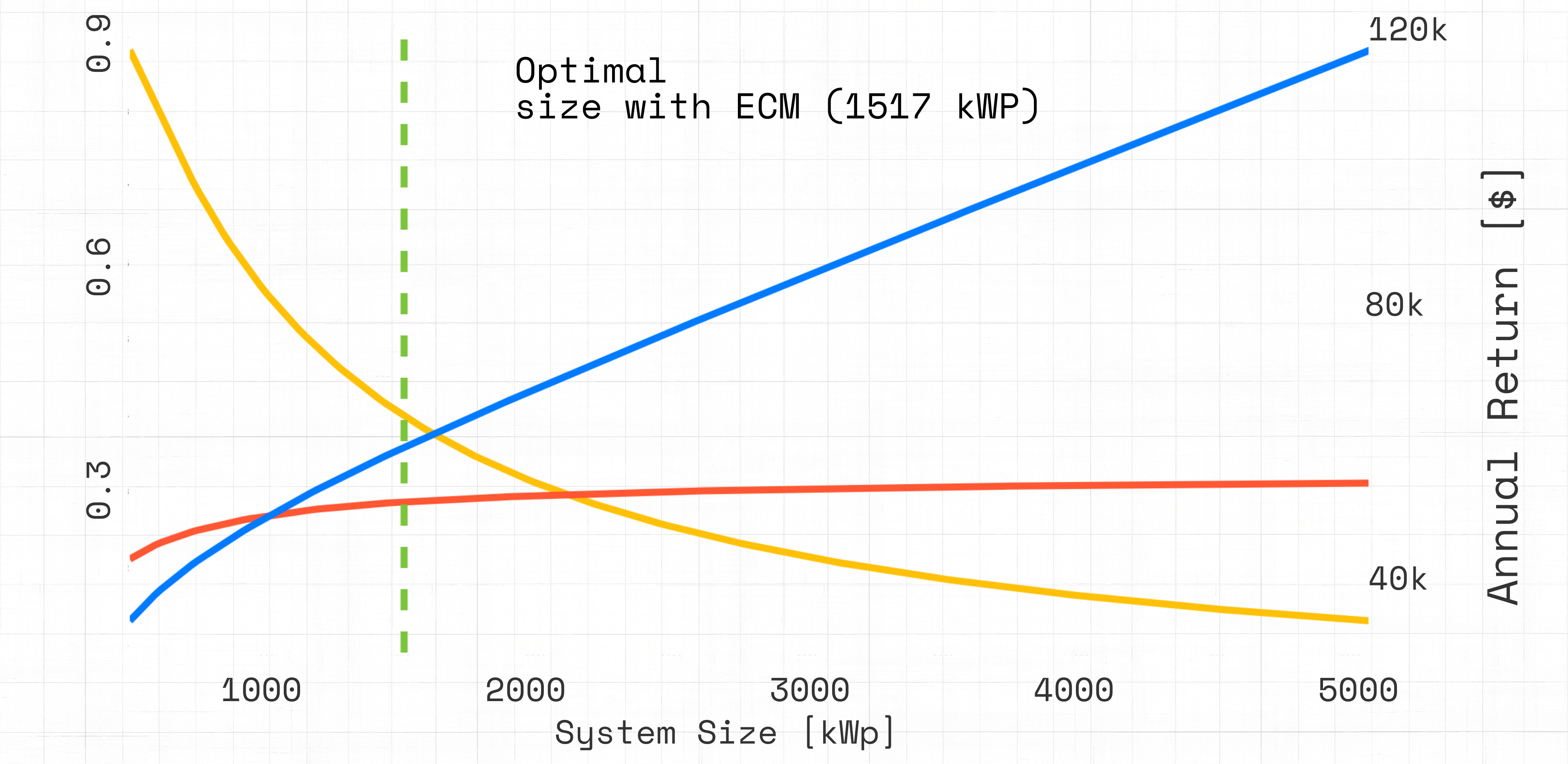
The profiles of the three curves change significantly before and after the ECM. We can notice a few things by analyzing the plot:
The optimal system size decreased, going from 1700 kWp to 1517 kWp
Before the ECM, the optimal system yielded a $97k annual return with 69% self-consumption and 27% self-sufficiency. After the ECM, it yields $60k, 40% self-consumption, and 29% self-sufficiency. This means that there was a 28% reduction in return and a 42% reduction in self-consumption for the optimal system.
The self-consumption ratio and annual return curves shifted significantly. For instance, if we stuck with a 1700 kWp system post-ECM, we’d only get $63k in return and 36% self-consumption.
While it’s straightforward that a lower overall consumption would lead to a smaller optimal system, the way in which the two curves shift is more nuanced. The shape of the annual $ return curve depends on the difference between the price of self-consumed energy and exported energy. If both prices were equal, the annual ROI line would be a simple linear function of system size. But when self-consumption is valued differently from injection into the grid, the relationship depends heavily on how well the production aligns with the building’s consumption. In the post-ECM case, the shape of the self-consumption ratio curve changed substantially because the ECM had a bigger impact during the hours that coincided with solar production. As we scale up the PV system, more energy ends up being exported to the grid rather than self-consumed.
We can plot the reduction in ROI as a function of the size of the system to get an even better idea of the dynamics:
# plot the % reduction in annual ROI for each system size
return_reduction = (post_ecm_results_df['total_return'] - results_df['total_return']) / results_df['total_return']

fig = go.Figure()
fig.add_trace(go.Scatter(x=post_ecm_results_df['system_size'], y=return_reduction, mode='lines', name='ROI Reduction', line=dict(color='#007BFF', width=10)))
fig.add_trace(go.Scatter(x=post_ecm_results_df['system_size'], y=self_consumption_reduction, mode='lines', name='Self-consumption Reduction', line=dict(color='#ffc107', width=10)))
fig.update_layout(
    xaxis_title="System Size [kWp]"
)
fig.show()
At smaller capacities, both the pre- and post-ECM scenarios are offsetting a large share of on-site consumption at the higher retail rate, so the difference in returns is minimal. As we move up to a medium-sized system, the pre-ECM building can still put more solar output toward meeting its relatively higher midday load, whereas the post-ECM building begins to export more electricity at a lower tariff—widening the gap in returns. Then, for very large systems, both scenarios end up exporting most of their solar production, so the return difference narrows again.
This quick analysis shows how a single ECM can radically change financial projections. If we installed a 1700 kWp system before the ECM implementation expecting an annual return of $97k, but ended up with only $63k instead, that would cause serious problems for many portfolio managers.
Furthermore, this highlights how difficult it is to plan an optimal decarbonization strategy for a real estate portfolio when every project you implement can reshape the ROI of subsequent projects. Solving this problem efficiently requires a powerful blend of computational tools and engineering creativity, and it’s a really interesting challenge to be working on. If you’re working on similar topics, I’d love to chat about different approaches—feel free to reply to this email or connect with me on LinkedIn!