Code Tutorial: Building a Counterfactual Energy Model for Savings Verification - Part 2

An analysis using data from the Building Data Genome Project 2

In the previous episode of this code tutorial, we analysed and processed the electricity consumption and weather datasets from real building located in Washington DC. In this second part of the tutorial, we’ll build a counterfactual energy consumption model and use that to estimate the energy efficiency savings achieved in the building.

As a first step, let’s import lightgbm, the library that we’ll use for the modeling.

import lightgbm

In the previous episode of the tutorial, we had identified the installation period of the energy efficiency project, and we used that installation period to split the data between a baseline dataset and a reporting dataset. Let’s quickly inspect them before getting started with the modeling. For all the following lines of code to work, it is necessary to first run the code from the last post.

baseline_df.head()

Output

reporting_df.head()

Output

For a quick summary of what the baseline and reporting period datasets represent, you can refer to this post.

We will now build a function that creates and returns a counterfactual energy model. The algorithm of choice for this application is a Gradient Boosting Decision Tree, built using the Python library lightgbm.

LightGBM stands out for its efficiency, speed, and accuracy, which have been widely demonstrated for tabular data applications. LightGBM was also part of the winning algorithm in the ASHRAE Great Energy Predictor III, a Kaggle competition aimed at developing data-driven models to predict energy use in buildings. According to the paper describing the results of the competition: "The most popular and accurate machine learning workflows used large ensembles of mostly gradient boosting tree models".

def build_baseline_model(data, target_variable, features, seed=None):

    data = data.dropna(subset=[target_variable])
    X = data[features]

    y = data[target_variable]
    dataset = lightgbm.Dataset(X, y)

    objective = "l2"
    lgbm_params = dict(
        boosting_type="gbdt",
        n_jobs=1,
        objective=objective,
        seed=seed or 42,
        verbosity=0,
    )
    cv = lightgbm.cv(
        params=lgbm_params,
        train_set=dataset,
        stratified=False,
        num_boost_round=200,
        nfold=5,
        callbacks=[lightgbm.early_stopping(5)],
    )

    # Full model (use best num-rounds from cross-validation)

    model = lightgbm.train(
        params=lgbm_params,
        train_set=dataset,
        num_boost_round=len(cv[f"valid {objective}-mean"]),
    )

    # Predict

    y_pred = pd.Series(model.predict(X), index=X.index)

    return {
        "data": data,
        "features": features,
        "target": target_variable,
        "seed": seed,
        "params": lgbm_params,
        "estimator": model,
        "cv": cv,
        "preds": y_pred,
    }

Let’s dig into some of the details of this function. The main idea is that we want to first split the provided dataset into explanatory features and target variable, and then fit a Gradient Boosting Decision Tree regression model using L2 as the loss function (objective). For regression tasks, L2 is equivalent to the mean squared error (MSE). 5-fold cross-validation is then used to find the optimal number of boosting iterations for the algorithm. Note here that, in favor of simplicity, some hyperparameters, such as the number of leaves of the trees or the learning rate, are not being optimized.

I do appreciate that not everyone might be familiar with the concepts of cross-validation or hyperparameter optimization, and I might write another post in the future to dig deeper on these topics. I decided to not explain them in detail here because they are the subject of a wide range of books, articles, and code examples.¹ My objective with this tutorial is to focus more on the concrete application in analysis than on the statistical nuances behind the modeling.

The next step is to use the defined build_baseline_model function to generate a counterfactual scenario and estimate the energy that would have been consumed in the absence of the energy-saving interventions. Comparing the counterfactual with the actual energy consumption recorded during the reporting period reveals the energy savings achieved due to the implemented energy efficiency project. Let’s define a function that can go through all of these steps and return the total verified energy savings, the adjusted baseline consumption time-series, and the baseline model used for the calculations.

def estimate_savings(baseline_df, reporting_df, target_variable):
    
    model_features = baseline_df.drop(
            target_variable, axis=1
        ).columns.to_list()

    baseline_model = build_baseline_model(baseline_df, target_variable=target_variable, features=model_features)

    adjusted_baseline = pd.Series(
            baseline_model["estimator"].predict(reporting_df[baseline_model["features"]]),
            index=reporting_df.index,
        )

    measured_reporting_data = reporting_df[target_variable]
    energy_savings = adjusted_baseline - measured_reporting_data
    total_energy_savings = round(energy_savings.sum())

    return total_energy_savings, adjusted_baseline, baseline_model

We can now apply the estimate_savings function to predict and visualize the total energy savings associated with the energy efficiency intervention in analysis.

total_energy_savings, adjusted_baseline, baseline_model = estimate_savings(baseline_df, reporting_df, 'consumption')

# Print total savings in kWh
print(f"Total estimated savings: {total_energy_savings} kWh")

Output

We have a result! Let’s build a visualisation that can help us better understand it.

# Results visualisation

# Resample consumption to daily frequency to improve clarity
baseline_daily = baseline_df.resample('1D').sum()
reporting_daily = reporting_df.resample('1D').sum()
adjusted_baseline_daily = adjusted_baseline.resample('1D').sum()

# build plot
fig = go.Figure()

fig.add_trace(go.Scatter(x=baseline_daily.index, y=baseline_daily['consumption'], line=dict(color='#007BFF')))

fig.add_trace(go.Scatter(x=adjusted_baseline_daily.index, y=adjusted_baseline_daily, line=dict(color="#7ac53c")))

fig.add_trace(go.Scatter(x=reporting_daily.index, y=reporting_daily['consumption'], line=dict(color='#007BFF')))

fig.add_trace(
        go.Scatter(
            x=adjusted_baseline_daily.index,
            y=adjusted_baseline_daily,
            mode="lines",
            showlegend=False,
            line=dict(color="rgba(135, 197, 95, 0.2)", width=0),
            fill="tonexty",
            fillcolor="rgba(135, 197, 95, 0.2)",
        )
    )

fig.update_layout(template='plotly_white', showlegend=False)

fig.add_vrect(x0=installation_start, x1=installation_end, fillcolor="#FF5733", opacity=0.3, line_width=0)

fig.show()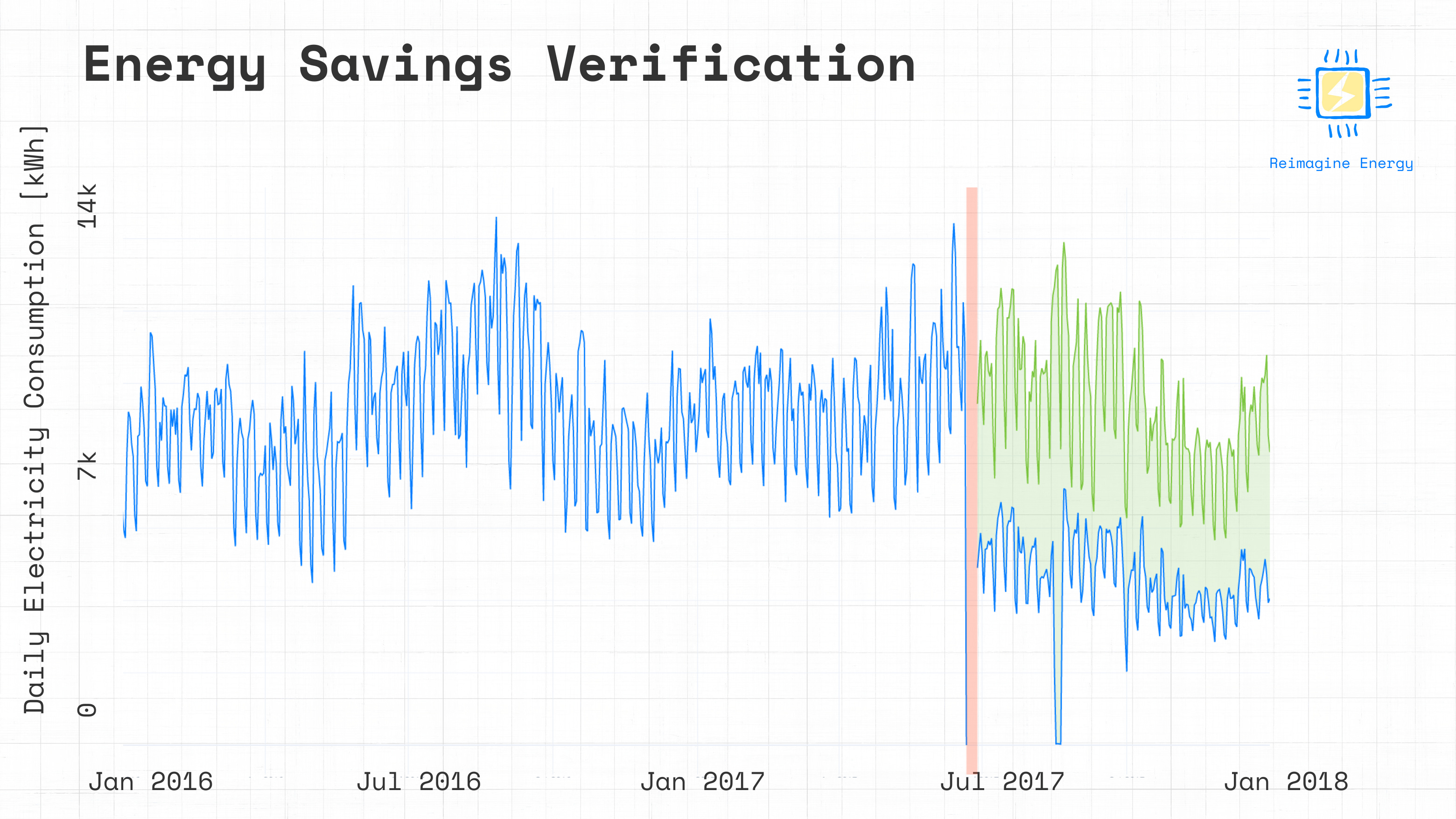

The resulting image shows the baseline and reporting periods, separated by a light orange band representing the installation period. The blue time-series represents the measured baseline and reporting period energy consumption, while the green time-series represents the adjusted baseline consumption predicted using our counterfactual energy model. The difference between the green and the blue line represents the estimated energy savings.

Conclusion

In the second part of this code tutorial, we built a counterfactual energy consumption model and estimated energy efficiency savings for a real building located in Washington DC. All of this was achieved with few, clean, lines of code, using the lightgbm library.

Although we have now reached a result, our analysis is not complete yet. You might have noticed that up to this point there was no mention of two fundamental aspects of Measurement & Verification: the interpretability of the counterfactual model, and the uncertainty of the estimated savings. We’ll dig deeper on these topics in the next episode!

1. To gain a deeper understanding of the Machine Learning part of this tutorial, I recommend starting with the chapter on decision trees from An Introduction to Statistical Learning. The lightgbm Python library documentation provides most of the knowledge required to use it, but the original whitepaper can be of interest as well for more hardcore readers.