Code Tutorial: Building a Counterfactual Energy Model for Savings Verification - Part 3

A journey in the land of uncertainty

Over the last few weeks, we’ve been looking at how to build a counterfactual energy model to verify energy efficiency savings using Python. In the first part of this code tutorial we accessed and preprocessed the data, while in the second we built the energy consumption model and used it to estimate the savings. In this post, the focus will be on how to quantify the uncertainty of the model-estimated savings.

Uncertainty quantification when estimating energy efficiency savings plays a key role, helping stakeholders understand the reliability of the predictions, better manage the risks associated with energy efficiency projects, and facilitate more informed decision-making processes.

In this tutorial, we’ll test two different techniques to quantify uncertainty: an approach included in the ASHRAE Guideline 14, and k-fold cross validation. Both techniques aim to quantify the uncertainty of the total estimated energy savings value, rather than the uncertainty of the savings estimation for each time step of the reporting period. These two methodologies were thoroughly compared within this article by Touzani et al., which I recommend reading in detail if you’re interested in the topic.

Let’s now explore the theory behind each technique and look at how to implement both methods using Python.

Method 1: ASHRAE Formula

The first method is based on a formula which is included in the ASHRAE Guideline 14. I introduced and discussed the formula in detail in a previous post, the main idea is that it correlates savings uncertainty with the model error (MSE), the number of baseline (n) and reporting (m) period observations, and the ratio between the total reporting period consumption (Epost) and the average baseline period consumption (Epre).

\(\Delta E_{save}^{ASHRAE} =1.26 \, t_{1-\alpha/2} \frac{E_{post}}{m \bar{E}_{pre}} \sqrt{MSE \, (1 + \frac{2}{n})\, m} \)

One important detail is that this formulation is based on the assumption that the only input variable considered in the regression model is outdoor temperature, and that the predictions are estimated with a linear regression model, using the ordinary least squares method (OLS). The model errors are also supposed to be independent and normally distributed.

Let’s create a Python function that can quantify the savings uncertainty using this formula.

In order for the following code snippets to work, the code from the previous two tutorials has to be run first.

import numpy as np

def calculate_ashrae_uncertainty(
    baseline_signal, adjusted_baseline_signal, baseline_model
):
    # calculate the uncertainty of the estimated savings at 95% confidence level using the formula
    derived from the ASHRAE Guideline 14

    measured_baseline = baseline_signal
    n = len(measured_baseline)
    m = len(adjusted_baseline_signal)
    mse = baseline_model["cv"]["valid l2-mean"][-1]

    # 1.26 is an approximated value that was found by Reddy and Claridge to eliminate the need of matrix algebra
    # in the calculation. 1.96 is the t-statistic value with 95% confidence level

    ashrae_uncertainty = (
        1.26
        * 1.96
        * adjusted_baseline_signal.sum()
        / m
        / measured_baseline.mean()
        * np.sqrt(mse * (1 + (2 / n)) * m)
    )

    return ashrae_uncertainty

Method 2: k-fold CV

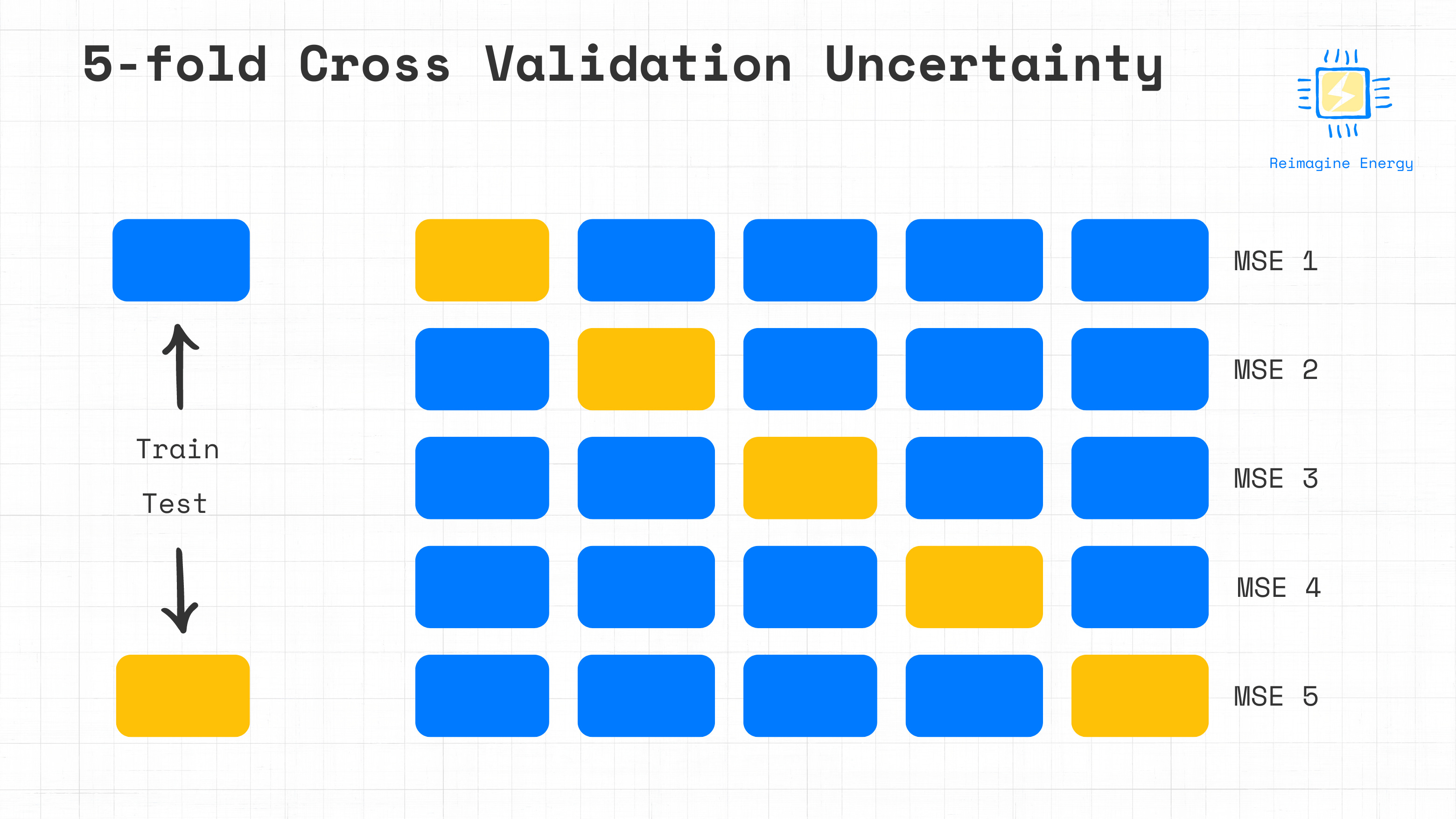
The second methodology proposed involves estimating the prediction error by using k-fold cross validation. The k-fold cross-validation method involves randomly dividing the training dataset (baseline period) into k subsamples, or folds, of approximately equal size. During the first iteration, the baseline model is built using k-1 folds as the training dataset, while the remaining fold (prediction set) is used to calculate the initial estimation of the prediction error. The uncertainty is assessed using the mean squared error (MSE) of the held-out fold, denoted as MSEi . This process is repeated k times, with a different fold serving as the test set in each iteration. An example with k=5 follows.

The final k-fold CV estimate of the MSE is obtained by averaging the MSEi values from all k iterations.

\(MSE^{CV} = \frac{1}{k} \sum^k_{i=1} MSE_i\)

Under the assumption that the errors are independent and normally distributed, the uncertainty of the total estimated energy savings can then be estimated as:

\(\Delta E^{CV}_{save}=z_{1-\alpha/2} \sqrt{m \ MSE^{CV}}\)

When training the baseline model, in the previous tutorial, we already performed 5-fold CV and saved the MSE values in the model results dictionary. Quantifying the uncertainty with 5-fold CV then becomes straightforward.

# calculate 5-fold cross validation uncertainty

def calculate_cv_uncertainty(adjusted_baseline_signal, baseline_model):

    mse_scores = baseline_model['cv'][f"valid l2-mean"]
    average_mse = np.mean(mse_scores)
    m = len(adjusted_baseline_signal)

    # 1.96 is the t-statistic value with 95% confidence level
    cv_uncertainty = 1.96 * np.sqrt(m * average_mse)
    
    return cv_uncertainty

Let’s run and compare the two methods now!

Comparison

A key distinction between the ASHRAE formulation and the k-fold CV method is that the k-fold CV method yields a non-deterministic estimate of uncertainty, whereas the ASHRAE method is deterministic. This means also that different trials of the k-fold CV method can produce varying estimates of the quantified uncertainty, if a seed is not set.

# Print and compare the uncertainty quantification results

ashrae_uncertainty = round(calculate_ashrae_uncertainty(baseline_df['consumption'], adjusted_baseline, baseline_model))

cv_uncertainty = round(calculate_cv_uncertainty(adjusted_baseline, baseline_model))

print(f'ASHRAE uncertainty results: Total savings = {total_energy_savings} +- {ashrae_uncertainty} kWh')
print(f'CV uncertainty results: Total savings = {total_energy_savings} +- {cv_uncertainty} kWh')

Output

The two methods align well in their estimated uncertainty, which is only about 0.5% of the projected savings. This suggests that the baseline period is sufficiently long for accurate estimation and that our model error is quite low. However, it’s worth questioning whether this extremely low uncertainty is realistic. Touzani’s study reveals two interesting findings:

1. When building models with high-resolution meter data (e.g., 15-minute, hourly, or daily) autocorrelated model errors appear. This means that the errors are not randomly distributed over time, and each error observation is not completely independent of others.

2. When testing the two methods over a large number of buildings, both tended to underestimate uncertainty, more so for hourly models than daily models due to stronger autocorrelation in hourly data.

While we can attempt to account for autocorrelation by modifying the number of independent observations (ASHRAE provides a guideline for this), the impact is not negligible. While the methods currently available provide a good initial estimate of uncertainty, they also appear to not be entirely reliable.

As of my knowledge, no superior method has been established, leaving it to our community of engineers, statisticians, and ML professionals to develop a better approach to quantify uncertainty in a more accurate way. The Efficiency Valuation Organization (EVO) has an uncertainty assessment application guide and is currently working on an update that might include valuable improvements on this front.